Decision Tree Mathematical Formulation

A decision tree is a tree where each internal node specifies a test on an attribute of the data in question and each edge between a parent and a child represents a decision or outcome based on that test.

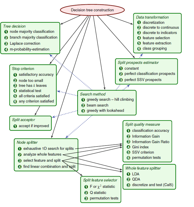
Fig. 1 Construction of Decision Tree and Information Flow in Decision Tree [1]

Following are the top-down approach of object-oriented analysis and design to determine components of the tree construction algorithm,

1. a search method that composes the tree node by node,
2. node splitter—a procedure responsible for splitting the nodes,
3. stop criterion—the rule that stops the search process,
4. split acceptor—the rule that decides whether to accept the best split of a node or to make it a leaf
5. split prospects estimator—a procedure that defines the order in which the nodes of the tree are
6. split—when using some stop criteria, the order of splitting nodes may be very important, but in most cases it is irrelevant
7. decision-making module which provides decisions for data items on the basis of the tree,
8. optional data transformations that prepare the training data at the start of the process or convert the parts of data at particular nodes.

·         NOTE  -  find more details about all the above steps in [1]

A sketch of dependencies between the modules is presented in Fig. 1. It can be viewed in terms of classes and interfaces: each box represents an interface and enumerates some classes implementing the interface. In the fig. 1, the solid arrows represent submodule relation while the dotted ones show the modules used by the search process. Such an amount of extracted interfaces and their implementations as depicted which is satisfactory for building a quite large number of DT induction algorithms including the most popular ones and many others.

A decision tree is a classifier. Decision trees are a widely used technique in statistical learning, where they are constructed to fit an existing set of data, and then used to predict outcomes on new data. We start with 𝑁 labeled “training records” of the form (𝑿,𝑌) where 𝑿 is a 𝑘-dimensional vector of features describing the data we have, and 𝑌 is a label we give this record. For example, our data may be characteristics about humans and our label may be their shoe size, so an example dataset could look like this

Each component of 𝑿 is called as “input variable”, 𝑌 is called “dependent variable” or “target variable”, and each row in such a table is called a “training example”. Let us consider two input variables, such that 𝑿=(𝑋1, 𝑋2). Further, let’s assume there is an interesting value of 𝑋1 that we can split the dataset around and few interesting values of 𝑋2. Then, an example partitioning of our space of (𝑋1, 𝑋2) values is depicted in the left side of Figure 2, and a decision tree corresponding to such a partitioning is shown in the right side of the figure. Given an unlabelled vector 𝑿 = (𝑋1, 𝑋2), we first test whether 𝑋1>𝑎. Then, if that turns out to be true, we test whether 𝑋2>𝑑. This allows us to classify 𝑿 into the region 𝑅4 or the region 𝑅5. If we initially had that 𝑋1≤𝑎, then we will test 𝑋2 against 𝑐 and then against 𝑏, which allows us to further classify 𝑿 into one of the regions 𝑅1,𝑅2, or 𝑅3.

fig. 2 a) partition of 2D space in five regions b) classifying decision tree into one of the five regions [1]

Next, let 𝑌 take on a single constant value for each of the regions 𝑅1,..,𝑅5. Let 𝑌𝑖 be the value chosen for the region 𝑅𝑖, and let 𝐼𝑖(𝑿) be an indicator function that equals 1 when 𝑿∈𝑅𝑖. This allows us to obtain a model that can predict 𝑌 based on 𝑿:

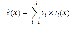
Obtaining such a model is the ultimate goal of training a decision tree. Same as the model represented in Fig. 2 as a partition of 2D space and as a decision tree.

The most basic process of training a decision tree on a dataset involves the following elements as,

1.       The selection of attribute

2.      Splits in the tree

3.      Stop splitting a node and mark it terminal

4.      The assignment of a label to each terminal node

Some algorithms add an element called pruning. There are many different ways of implementing splitting criteria, stopping criteria, and pruning methods. Splitting criteria are algorithmic rules that decide which input variable to split the dataset around next. Stopping criteria are rules that determine when to stop splitting the dataset and instead output a classification. Stopping criteria are actually optional, but in their absence, a trained tree would have a separate region for each training record. As this is undesirable, stopping criteria are used as a method of deciding when to stop growing the tree. Lastly, pruning methods are ways to reduce the size and complexity of an already trained tree by combining or removing rules that do not significantly increase classification accuracy. All three of these things directly affect the complexity of a tree, which can be measured according to various metrics such as tree height, tree width, and a number of nodes. It is desirable to train trees that are not overly complex because of the fact that simpler trees require less storage.

We now begin a description of several splitting criteria. In particular, we will discuss splitting criteria that only consider the values of a single input variable. Such criteria are called univariate splitting criteria. For a given dataset of training records D of the form (𝑿, 𝑌), we let 𝑇𝑖 be a test on a record that considers the attribute 𝑋𝑖 and has n outcomes 𝑂1, 𝑂2…𝑂𝑛. An example of such a test would be 𝑋1>𝑎 which has two outcomes. Many different tests could exist for each input attribute. A given test will split the dataset D into 𝑛 different subsets 𝐷1, 𝐷2…𝐷𝑛. The following is a generic tree training algorithm.

Algorithm: Train Tree Input: D, a dataset of training records of the form (X, Y). Output: Root node R of a trained decision tree 1) Create a root node R 2) If a stopping criterion has been reached then label R with the most common value of 𝑌 in 𝐷 and output R 3) For each input variable 𝑋𝑖 in X a.    Find the test 𝑇𝑖 whose partition 𝐷1, 𝐷2…𝐷𝑛 performs best according to the chosen splitting metric. b.    Record this test and the value of the splitting metric 4) Let 𝑇𝑖 be the best test according to the splitting metric, let 𝑉 be the value of the splitting metric, and let 𝐷1, 𝐷2… 𝐷𝑛 be the partition. 5) If 𝑉<𝑡ℎ𝑟𝑒𝑠ℎ𝑜𝑙𝑑 a.    Label R with the most common value of 𝑌 in 𝐷 and output R 6) Label R with 𝑇𝑖 and make a child node 𝐶𝑖 of R for each outcome 𝑂𝑖 of 𝑇𝑖. 7) For each outcome Oi of 𝑇𝑖 a.    Create a new child node 𝐶𝑖 of R, and label the edge 𝑂𝑖 b.    Set С𝑖 = Train Tree(𝐷𝑖) 8) Output R

Before we consider any individual splitting criterion, we need to define the notion of an impurity function, which is a start to understanding how well a given split organizes the dataset. An impurity function of a probability distribution 𝑃 is a function 𝜙:𝑃→ℝ that satisfies a few constraints:

1.       𝜙 attains its maximum if and only if 𝑃 is a uniform distribution.

2.      𝜙 attains its minimum if and only if some 𝑝𝑗=1 for some 𝑝𝑗∈𝑃

3.      𝜙 is symmetric about the components of 𝑃

4.      𝜙(𝑃)≥0 for all 𝑃

The application to decision trees arises from the fact that at each node, when considering a split on a given attribute we have a probability distribution 𝑃 with a component 𝑝𝑗 for each class 𝑗 of the target variable 𝑌. Hence we see that a split on an attribute it most impure if 𝑃 is uniform, and is pure if some 𝑝𝑗=1, meaning all records that past this split are definitely of class 𝑗. Once we have an impurity function, we can define an impurity measure of a dataset D node 𝑛 as so. If there are 𝑘 possible values 𝑦1,𝑦2,…,𝑦𝑘 of the target variable 𝑌, and 𝜎 is the selection operator from relational algebra then the probability distribution of 𝑆 over the attribute 𝑌 is

And the impurity measure of a dataset D is denoted as,

Lastly, we define the goodness-of-split (or change in purity) with respect to an input variable 𝑋𝑖 that has 𝑚 possible values 𝑣1,..𝑣𝑚 and a dataset 𝐷 as,

Impurity based splitting criteria use an impurity function 𝜙 plugged into the general goodness-of-split equation defined above.

Information Gain

Information gain is a splitting criterion that comes from information theory. It uses information entropy as the impurity function. Instead of the usual definition of information entropy as a function of a discrete random variable, we use a very similar definition of information entropy as a function of a probability distribution. This allows us to use it as our impurity function. Given a probability distribution 𝑃= (𝑝1, 𝑝2...𝑝𝑛), where 𝑝𝑖 is the probability that a point is in the subset 𝐷𝑖 of a dataset 𝐷, we define the entropy 𝐻:

Plugging in 𝐸𝑛𝑡𝑟𝑜𝑝𝑦 as our function 𝜙 gives us 𝐼𝑛𝑓𝑜𝑟𝑚𝑎𝑡𝑖𝑜𝑛𝐺𝑎𝑖𝑛𝑌 (𝑋𝑖, 𝐷):

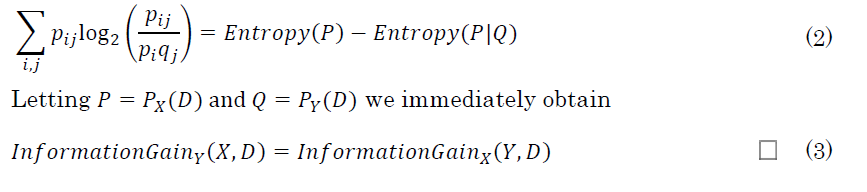
We can also define information gain as a function of conditional entropy. Suppose 𝑃 and 𝑄 are two distributions with 𝑛 and 𝑚 elements, respectively. The outcomes of the splits on 𝑃 and 𝑄 form a table 𝑇 where the entry 𝑇𝑖𝑗 contains the number of records in the dataset that survive both the 𝑃𝑖 split and the 𝑄𝑗 split. We let 𝑝𝑖𝑗=𝑇𝑖𝑗|𝐷|

Then conditional entropy is the entropy of a record surviving the split 𝑄 given that it survived 𝑃 as follows. We restrict the 𝑄 distribution to the column of 𝑇 that contains the result of the split on 𝑃, and then average over all possible splits on 𝑃.

Plugging in the definition for conditional entropy into the above immediately yields the equation for information gain presented earlier. We can now prove an interesting property of information gain, showing that when using this splitting criterion we cannot make negative progress in classifying data under our target attribute.

PROPOSITION 1: Information Gain is non-negative.

PROOF: This follows pretty easily from Jensen’s inequality since –𝑙𝑜𝑔(𝑥) is convex.

Jensen’s inequality states that 𝜑(𝐸[𝑋])≤𝐸[𝜑(𝑋)], where 𝑋 is a random variable, 𝐸 is the expectation, and 𝜑 is a convex function.

Letting 𝑃=𝑃𝑋𝑖(𝐷) and 𝑄=𝑃𝑌(𝐷) we get that splitting a dataset 𝐷 on an input variable 𝑋𝑖 yields non-negative information gain with respect to a target variable 𝑌. The result of this proof seems to say that splitting on any variable should not make the model any worse, since information gain is non-negative. However, this is not entirely true because overfitting may occur.

PROPOSITION 2: Information Gain is symmetric, meaning that if we switch the split variable and target variable, we still get the same amount of information gain. Expressed in our notation as:

PROOF: In step (5) of the proof of Proposition 1 showed that

Since this expression is symmetric around 𝑝𝑖 and 𝑞𝑗 it follows that

One issue with using information gain as a splitting criterion is that it is biased towards tests that have many outcomes [9]. For example, suppose we are building a decision tree on a dataset of customers, to be able to predict some form of customer behavior in the future. If one of the input attributes is something unique to each customer, such as a credit card number, phone number, social security number, or any other form of ID, then the information gain for such an attribute will be very high. As a result, a test on this attribute may be placed near the root of the tree. However, testing on such attributes will not extend well to records outside of the training set, which in this case are new customers, since their unique identifiers will not be an outcome of the test.

Gain Ratio

As a result, Quinlan proposes a related splitting criterion, called Gain Ratio or Uncertainty Coefficient [9]. This serves to normalize information gain on an attribute Xi relative how much entropy this attribute has.

We can clearly see that in the preceding example with customer data, the denominator will be very large. Since the identifiers are unique, the denominator would be on the order of the number of customers in the dataset, whereas the numerator is at most the number of possible values for 𝑌. However, it must be noted that if 𝐸𝑛𝑡𝑟𝑜𝑝𝑦 (𝑃𝑋𝑖(𝐷)) is very small, then this gain ratio will be large but 𝑋𝑖 may still not be the best attribute to split on. Quinlan suggests the following procedure when using gain ratio as the criterion:

1.         Calculate information gain for all attributes, and compute the average information gain

2.     Calculate the gain ratio for all attributes whose information gain is greater or equal to the average information gain, and select the attribute with the largest gain ratio

Quinlan claims that this gain ratio criterion tends to perform better than the plain information gain criterion, creating smaller decision trees. He also notes that it may tend to favor attributes that create unevenly sized splits where some subset 𝐷𝑖 of 𝐷 in the resulting partition is much smaller than the other subsets.

Gini Index

The Gini Index is another function that can be used as an impurity function. It is a variation of the Gini Coefficient, which is used in economics to measure the dispersion of wealth in a population [10]. It was introduced as an impurity measure for decision tree learning by Breiman in 1984. It is given by this equation

𝐺𝑖𝑛𝑖(𝐷) will be zero if some 𝑝𝑖=1 and it since each 𝑝𝑖<1, it will be maximized if all 𝑝𝑖 are equal. Hence we see that the Gini Index is a suitable impurity function. The Gini Index measures the expected error if we randomly choose a single record and use it’s value of Y as the predictor, which can be seen by looking at the second formulation of the Gini Index, 1−Σ(𝑝𝑖)2𝑛𝑖=1. This can be interpreted as a difference between the norms of the vectors (1…1) and 𝑃𝑦 (𝐷). Also, in the first formulation, Σ𝑝𝑖(1−𝑝𝑖)𝑛𝑖=1, it is simply the sum of 𝑛 variances of 𝑛. Bernoulli random variables, corresponding to each component of the probability distribution 𝑃𝑌(𝐷). We define the goodness-of-split due to the Gini Index similar to what we did with information gain, by simply plugging in 𝜙(𝐷)= 𝐺𝑖𝑛𝑖𝑌(𝐷) to obtain

It turns out that the Gini Index and information entropy are related concepts. Fig. 3 shows that they graphically look similar:

Fig. 3 Entropy and Gini Index graphed for two different values of J, which is the total number of classes of the target variable [3].

Misclassification Rate

Given a probability distribution 𝑃 we define the misclassification rate to be 𝑀𝑖𝑠𝑐𝑙𝑎𝑠𝑠𝑖𝑓𝑖𝑐𝑎𝑡𝑖𝑜𝑛(𝑃)=1−max𝑗𝑝𝑗 𝑤ℎ𝑒𝑟𝑒 𝑃=(𝑝1,…,𝑝𝑛) Again, it is easy to see that 𝑀𝑖𝑠𝑐𝑙𝑎𝑠𝑠𝑖𝑓𝑖𝑐𝑎𝑡𝑖𝑜𝑛 is indeed an impurity function. It is maximized when 𝑃 is uniform and it is zero when some 𝑝𝑗=1. We then define 𝑀𝑖𝑠𝑐𝑙𝑎𝑠𝑠𝑖𝑓𝑖𝑐𝑎𝑡𝑖𝑜𝑛𝐺𝑎𝑖𝑛 by plugging in 𝜙(𝑃)=𝑀𝑖𝑠𝑐𝑙𝑎𝑠𝑠𝑖𝑓𝑖𝑐𝑎𝑡𝑖𝑜𝑛(𝑃) into the goodness-of-split equation.

An interesting fact is that the Gini Index and the Misclassification Rate have the same maximum. Given that 𝑃 has 𝑛 elements, meaning that there are 𝑛 possible values of the target variable, the maximum Misclassification Rate is 1−1𝑛 and the maximum Gini Index is

1−𝑛∗(1/𝑛)² = 1−(1/𝑛).

Since the Gini Index and Entropy impurity functions are both differentiable, they are preferred over the Misclassification Rate where Differentiability helps with numerical optimization techniques.

Other Splitting Criteria

There are many other splitting criteria that one can use, and a good overview of these is in chapter 9 of the Data Mining and Knowledge Discovery Handbook While we have only considered univariate splitting criteria, this book has a brief description of multivariate splitting criteria as well.

Stopping Criteria

Stopping criteria are usually not as complicated as splitting criteria. Common stopping criteria include:

1.       Tree depth exceeds a predetermined threshold

2.      Goodness-of-split is below a predetermined threshold

3.      Each terminal node has less than some predetermined number of records

Generally stopping criteria are used as a heuristic to prevent overfitting. Overfitting is when a decision tree begins to learn noise in the dataset rather than structural relationships present in the data. An over-fit model still performs very well in classifying the dataset it was trained on, but would not generalize well to new data, just like the example with credit card numbers or other unique identifiers. If we did not use stopping criteria, the algorithm would continue growing the tree until each terminal node would correspond to exactly one record.

Conclusion

We have studied a general method of growing a decision tree using a greedy algorithm, with interesting analyses of several splitting criteria that can be used with this algorithm.

References

1. J. Kacprzyk, Warsaw, Poland, "meta learning in decision tree induction" springer vol 498
2. Lev dubinets “top-down decision tree inducers ”
3. Jugal Kalita, Decision and Regression Tree Learning. Slides. Used for figure 3. http://www.cs.uccs.edu/~jkalita/work/cs586/2013/DecisionTrees.pdf