Perceptron Model

A computer program is said to 'learn' from experience E with respect to some class of tasks T and performance measure P, if its performance at tasks in T, as measured by P, improves with experience E.

PROGRAMMING LANGUAGE

Python 3.6 version of the language is used in the blog codes. The main reason for a new version of Python is to remove all the small problems and nit-picks that have accumulated over the years and to make the language cleaner. If you already have a lot of Python 2.x code, then there is a utility to assist you to convert 2.x to 3.x source. According to me best book to learn python language is “PYTHONCRASH COURSE a hands on, project based introduction to programming” written by Eric Matthes, available online

INTRODUCTION

Machine learning is field of computer science that uses statistical techniques to give computer system the ability to ‘learn’ (i.e. successively improve performance on an original task) with data, without being comprehensibly programmed. Most sciences are empirical in nature, and this means their theories are based on robust empirical phenomena, such as the law of combining volumes and the ideal gas law. A growing number of machine learning researchers are focusing their efforts on discovering analogous phenomena in the behaviour of learning systems, and this is an encouraging sign.

In machine learning, the perceptron is an algorithm for supervised learning of binary classifiers (task of classifying the elements of a given set into two groups on the basis of classification rule.),the perceptron is the first artificial neural network.The artificial neural networks implement a computational paradigm inspired by the anatomy of the brain. The corresponding algorithms simulate simple processing units (called neurons) linked through a complex web of connections. This enables the networks to process separately different pieces of information while keeping into account their mutual constraints and relationships.

HISTORY

In considering the history of the perceptron it is important to note that the formal perceptron definition has only recently begun to stabilize. Given this lack of definitional stability (even Rosenblatt himself changed his definitions multiple times), this history section will simply mention a number of main influences on the development process. This is not really satisfactory, but it is probably the best that can be done short of a book length historical treatment (for a more extensive discussion see [Anderson and Rosenfeld, 1998]).

The idea that it might be possible to consider mathematical models of biological neurons goes back many decades [Anderson and Rosenfeld, 1988]. Before 1940, some attempts were made to mathematically model neural function, but none of these models were compelling. The first breakthrough came in 1943 with the seminal paper of McCulloch and Pitts [McCulloch and Pitts, 1943]. They postulated that neurons functioned as Boolean logic devices. While the logic circuit idea of McCulloch and Pitts was soon discredited as a biological theory, their work, and that of several others, led to a model of a neuron as a linear or affine sum followed by an activation function(usually a unit

step function with a threshold offset). This neuron model (which, over time, began to be frequently, but incorrectly attributed directly to McCulloch and Pitts) was widely adopted as a model for neuron behaviour.

The thinking stimulated by McCulloch and Pitts and those they inspired didn’t lead immediately to any important new concrete ideas, but it did generate a widespread feeling among prominent exponents of automated information processing (e.g., Norbert Weiner and John von Neumann, and many others) that building ‘artificial brains’ might become possible someday ‘soon’. This excitement became even greater in 1949 with the publication of Hebb’s hypothesis [Hebb 1949] that neuronal learning involves experience induced modification of synaptic strengths. Incorporating this hypothesis into the formal neuron (i.e. variable weights) created many new avenues of possible investigation.

Although many investigations were launched in the early 1950s into neural networks composed offormal neurons with variable (Hebbian) weights, none of them yielded significant results until about 1957. At that point, two disparate themes emerged which, astoundingly, have still not been reconciled or connected, the learnmatrixand the perceptron. Studies of the learnmatrix associative memory neural network architecture were launched by Karl Steinbuch in about 1956 and led in 1961 to his writing of Automat und Menschthe first technical monograph on artificial neural networks [Steinbuch, 1961, Steinbuch and Piske, 1963].

The perceptron (a term originally coined to mean a single threshold logic neuron designed to carry out a binary i.e., two-class pattern recognition function) was developed by Frank Rosenblatt beginning in 1956. By 1957 he had developed a learning method for the perceptron and was soon able to prove mathematically that, in the case of linearly separable classes, the perceptron would be able to learn, by means of a Hebb-style supervised training procedure, to carry out its linear pattern classification function optimally. For the first time, a formal neuron with trainable Hebbian weights was shown to be capable of carrying out a useful ‘cognitive’ function.

Because of the limitations of digital computers in the 1950s, Rosenblatt was initially unable to try out his ideas on practical problems. So he and his colleagues successfully designed, built and demonstrated a large analog circuit neurocomputer to enable experiments His machine (called the Perceptron Mark I) had 512 adjustable weights and a crude 400-pixel camera as its visual sensor. It successfully demonstrated an ability to recognize alphabetic characters. Rosenblatt’s work (which was widely publicized, including numerous popular magazine articles and appearances on major network television programs) inspired a large number of investigators to begin work on neural networks.

  Frank Rosenblatt, c 1959 Photographed

in connection with a television appearance 

with the "eye" of the Perceptron Mark I

Pic Courtesy: Wiki

By 1962, Rosenblatt’s book (the second monograph on neural networks) Principles of Neurodynamics[Rosenblatt, 1962] discussed a more advanced sort of perceptron one similar to that discussed in thisbook. However, a big unsolved problem remained an effective method for training the hidden layerneurons.

Another important development of the late 1950s was the development of the ADALINE(ADAptiveLINearNEuron – but it was actually affine) by Widrow and Hoff [Widrow and Hoff, 1960]. The learning law for this network was the delta rule used in the output layer neurons of the perceptron. Widrow’s perspicuous mathematical derivation of the delta rule learning law set the foundation for many important later developments. As with Rosenblatt, Widrow turned to analogelectronics to build an implementation of the ADALINE (including development of a variable-electrical resistance weight implementation device called a MEMISTOR [Hecht-Nielsen, 1990]).

A development which was understood only by a few experts at the time, but which is now recognized as a phenomenally prescient insight, was the discovery in 1966 of the essential part of the generalized delta rule by Amari [Amari, 1967]. The only thing missing was how to calculate the hidden neuron errors.

By the mid-1960s many of the researchers who had been attracted to the field in the late 1950s began to become discouraged. No significant new ideas had emerged for some time and there was no indication that any would for a while. Many people gave up and left the field. Contemporaneously, a series of coordinated attacks were lodged against the field in talks at research sponsor headquarters, talks at technical conferences and talks at colloquia. These attacks took the form of rigorous mathematical arguments showing that the original perceptron and some of its relatives were mathematically incapable of carrying out some elementary information processing operations (e.g., the Exclusive-OR logical operation). By considering several perceptron variants and showing all of them to be ‘inadequate’ in this same way, an implication was conveyed that all neural networks were subject to these severe limitations. These arguments were refined and eventually published as a book [Minsky and Papert, 1969] (see [Anderson and Rosenfeld, 1998] for a more thorough discussion). The final result was the emergence of a pervasive conventional wisdom (which persisted until 1985) that ‘neural networks have been mathematically proven to be useless’.

Although the missing piece of the generalized delta rule (i.e., backpropagation) was independentlydiscovered by at least two people during the period 1970-1985 [Anderson and Rosenfeld, 1998], namely Paul Werbos in 1974 and David Parker in 1982, these discoveries had little impact and did not becomewidely known until after the work of Rumelhart, Hinton, and Williams in 1985 [Rumelhart et al 1986]. As can be seen by referring to any current text on neural networks (e.g., [Haykin, 1999 Fine, 1999]), enormous progress has occurred since then. The faith that Rosenblatt (who died in a boating accident in 1971) had in the perceptron has been resoundingly vindicated. 

Charles Wightman holding a subrack of eight

perceptron adaptive weight implementation units

Pic Courtesy: Veridian Engineering

DEFINITION

Definition: It’s a step function based on a linear combination of real-valued inputs. If the combination is above a threshold it outputs a 1, otherwise it outputs a –1.

Fig. 3 Perceptron Model

O(x_1,x_2,..,x_n) =1 or -1

Output is 1 if w₀+w₁x₁+w₂x₂+....+w_nx_n ≥0 otherwise -1

where

x_1,x_2,..,x_n= input vector

w_1, w_2,..,w_n= weight vector

A perceptron draws a hyperplane as the decision boundary over the (n-dimensional) input space.

Fig. 4 Decision boundry over the input space

A perceptron can learn only examples that are called “linearly separable”. These are examples that can be perfectly separated by a hyperplane.

Fig. 5 Graphical from of Linearly separable and Non-linearly separable

Perceptrons can learn many boolean functions: AND, OR, NAND, NOR, but not XOR

However, every boolean function can be represented with a perceptron network that has two levels of depth or more.

Perceptron Learning

Learning algorithms can be divided into supervised and unsupervised methods. Supervised learning denotes a method in which some input vectors are collected and presented to the network. The output computed by the network is observed and the deviation from the expected answer is measured. The weights are corrected according to the magnitude of the error in the way defined by the learning algorithm. This kind of learning is also called learning with a teacher, since a control process knows the correct answer for the set of selected input vectors. Unsupervised learning is used when, for a given input, the exact numerical output a network should produce is unknown. Supervised learning is further divided into methods which use reinforcement or error correction. Reinforcement learning is used when after each presentation of an input-output example we only know whether the network produces the desired result or not. The weights are updated based on this information (that is, the Boolean values true or false) so that only the input vector can be used for weight correction. In learning with error correction, the magnitude of the error, together with the input vector, determines the magnitude of the corrections to the weights, and in many cases we try to eliminate the error in a single correction step.

Fig. 6 classes of learning algorithms

The perceptron learning algorithm is an example of supervised learning with reinforcement. Some of its variants use supervised learning with error correction (corrective learning).

Learning a perceptron means finding the right values for W. The hypothesis space of a perceptron is the space of all weight vectors. The perceptron learning algorithm can be stated as below. Learning algorithm is explained in sentence form and mathematical formate.

1. Assign random values to the weight vector

2. Apply the weight update rule to every training example

3. Are all training examples correctly classified?

a. Yes. Quit

b. No. Go back to Step 2.

There are two popular weight update rules.

i) The perceptron rule, and

ii) Delta rule

OR

We are now in a position to introduce the perceptron learning algorithm. The training set consists of two sets, P and N, in n-dimensional extended input space. We look for a vector w capable of absolutely separating both sets, so that all vectors in P belong to the open positive half-space and all vectors in N to the open negative half-space of the linear separation

1.      Start : The weight vector w0 is generated randomly, 

Set t = 0

2.      test: A vector x ∈ P ∪ N is selected randomly,

a.       if x∈P and w.x>0 go to test,

b.      if x∈P and w.x≤0 go to add,

c.       if x∈N and w.x< 0 go to test,

d.      if x∈N and w.x≥0 go to subtract.

3.      add: set wt+1= w_t+x and t=t+1 go to test

4.      subtract: set wt+1= w_t-x and t= t+1 go to test

This algorithm makes a correction to the weight vector whenever one of the selected vectors in P or N has not been classified correctly. The perceptron convergence theorem guarantees that if the two sets P and N are linearly separable the vector w is updated only a finite number of times. The routine can be stopped when all vectors are classified correctly. The corresponding test must be introduced in the above pseudocode to make it stop and to transform it into a fully-fledged algorithm

     The Perceptron Rule 

      For a new training example X=(x_1,x_2,..,x_n) update each weight according to this rule:w_i=w_i+Δw_i

       Where

      Δw_i=-η(t-o)x_i

         t = target output

         o = output generated by the perceptron

         η = constant called the learning rate (e.g., 0.1)

         Comments about the perceptron training rule

• If the example is correctly classified the term (t-o) equals zero, and no update on the weight is necessary.

• If the perceptron outputs –1 and the real answer is 1, the weight is increased.

• If the perceptron outputs a 1 and the real answer is -1, the weight is decreased. 

• Provided the examples are linearly separable and a small value for η is used, the rule is proved to classify all training examples correctly (i.e, is consistent with the training data). 

Execution of Code Step By Step

Perceptron is linear classifier (binary). It is used in supervised learning. It helps to classify the given input data. One can see it has multiple stage of execution as below

1. Input Values

2. Weights and Bias

3. Net sum

4. Activation Function

Why we need weights and biases? Weights shows the strength of the particular node. A bias value allows you to shift the activation to the left or right. Why we need activation function? The activation function are used to map the input between the required values lie (0,1) or (-1,1). The machine learning algorithms work as the perceptron model in neural network. Learning the basic of perceptron model will help to understand rest of machine learning algorithms. Let us see code execution in steps.

ASSUMPTIONS

1.      Perceptrons can only converge on a linearly separable inputs.

2.      Perceptrons learning procedure can only be applied to a single layer of neurons.

3.      Perceptrons  can only learn online, because the perceptron learning is based on the error of binary classifier (error can be -1,0 or 1)

DATA

Dataset comes from the UCI Machine Learning Repository and it is related to Iris plant database containing flower classes setosa, versicolor and virginica. Attributes are sepal length and sepal width, petal length and petal width.

Step 1

Iris dataset have labels and raw data which is unsupervised. Import this data set using Sklearn library. Print the iris data find what the output is. Total number of instances are 150 i.e first 50 Iris_setosa, next 50 Iris_vesicolour and remaining 50 areIris_ virginica.

Output

Step 2

Selection of class and attributes i.e from the class we are going to select Iris_versicolour and Iris_verginica i.e data from 50-150 and selected class attributes are sepal width and petal length.

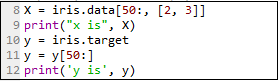
Output

Step 3

Training and splitting the data. Usually data is split into training data and test data.

 Fig. 7 splitting of data into train and test datasets. 

Training set contains a known output and the model learn on this data in order to generalize to other data later on. Use test dataset (subset) in order to test model’s prediction on the subset. For splitting data sklearn library is used as “from sklearn.model_selection import train_test_split” Here data is split into training 80% and test data 20% i.e test_size = 0.2

Step 4

In statistics and machine learning the term Data standardisation is very important. Usually data is split into two subsets training and test datasets (sometime it split into three data set train, validate and test) and fit model on train dataset in order to make prediction on test dataset. While in prediction two possibilities can happen overfit of model and underfit of model. Which is avoided to happen. Will see what exactly overfit and underfit actually mean with data standardisation afterwords. Now predict and fit the data. Here training data must be predict, fit and transform but test data is only predict and transform. For data standardisation use “from sklearn.preprocessing import StandardScaler”

 Step 5

Now use the perceptron model from “from sklearn.linear_model import Perceptron” to check the misclassifications of chosen class and attributes.

Where

n_iter = The number of passes over the training data (aka epochs). Defaults to 5.

eta0 = Constant by which the updates are multiplied. Defaults to 1.

Now print ppn.fit and y_pred check the output.

Output